當AI遇上股票
台南一中AI選修教材 / 顏永進
Table of Contents

以下範例均假設於Google Colab上執行,若於本機IDE(如PyCharm、Spyder)上執行,則部份指令執行方式要略做修正。
1. CNN-1: 以AI預測股價-隔日漲跌
1.1. 安裝相關套件
1: pip install yfinance
1.2. 下載股價資訊
1: import yfinance as yf
2:
3: df = yf.Ticker('2330.TW').history(period='10y')
4: print(type(df))
1.2.1. 查看下載的資料集
1: print(df[:5])
1.2.2. 取出需要的收盤價
從陣列中讀出收盤價
1: data = df.filter(['Close'])
2: print(data.head())
1.3. 觀察原始資料/日K圖
1: import matplotlib.pyplot as plt
2: plt.clf()
3: plt.plot(data.Close)
4: plt.show()
1.4. 將資料標準化
1: from sklearn.preprocessing import MinMaxScaler
2: scaler = MinMaxScaler(feature_range=(0, 1))
3: sc_data = scaler.fit_transform(data.values)
4:
5: sc_data #變成numpy array
1.5. 建立、分割資料
1.5.1. 建立資料集及標籤
 1: import numpy as np
 2:
 3: # 以前N天的股價來預測未來股價
 4: previousNDays = 10
 5: x_data, y_data = [], []
 6: for i in range(len(sc_data) - previousNDays):
 7:   x = sc_data[i:i+previousNDays]
 8:   y = sc_data[i+previousNDays]
 9:   x_data.append(x)
10:   y_data.append(y)
11: #因為等一下要送進tensorflow,所以先轉成numpy的陣列格式
12: x_data, y_data = np.array(x_data), np.array(y_data)
13:
14: print(x_data.shape)
15: print(y_data.shape)
1.5.2. 分割訓練集與測試集
 1: ratio = 0.8
 2: train_size = round(len(x_data) * ratio)
 3: print(train_size)
 4: # 第0筆到第train_size-1筆的資料分割為訓練集
 5: x_train, y_train = x_data[:train_size], y_data[:train_size]
 6: # 第train_size筆到最後一筆的資料分割為測試集
 7: x_test, y_test = x_data[train_size:], y_data[train_size:]
 8: #from sklearn.model_selection import train_test_split
 9: #x_train, x_test, y_train, y_test = train_test_split(x_data, y_data, test_size=0.2)
10: print(x_train.shape)
11: print(y_train.shape)
12: print(x_test.shape)
13: print(y_test.shape)
1.6. 建立、編譯、訓練模型
1.6.1. 建立模型
 1: # CNN模型
 2: import tensorflow as tf
 3: from tensorflow.keras import layers
 4:
 5: #建構CNN模型
 6: model = tf.keras.Sequential([
 7:     layers.Input(shape=(previousNDays, 1, 1)),
 8:     #卷積層:用 3 天的窗格掃描股價模式
 9:     layers.Conv2D(filters=512, kernel_size=(3, 1), activation='relu'),
10:     #攤平
11:     layers.Flatten(),
12:     #全連接層/輸出層(回歸問題不加激活函數)
13:     layers.Dense(1)
14: ])
1: model.summary()
1.6.2. 編譯模型
1: model.compile(loss='mse', optimizer='adam', metrics=['mae'])
1.6.3. 訓練模型
1: model.fit(x_train, y_train,
2:           validation_split=0.2,
3:           batch_size=200, epochs=20)
1.7. 性能測試
1.7.1. loss
1: score = model.evaluate(x_test, y_test)
2: print('loss:', score[0])
3: print('mae:', score[1])
1.7.2. predict
1: predict = model.predict(x_test)
2: predict = scaler.inverse_transform(predict)
3: predict = np.reshape(predict, (predict.size,))
4: ans = scaler.inverse_transform(y_test)
5: ans = np.reshape(ans, (ans.size,))
6: print(predict[:3])
7: print(ans[:3])
1.7.3. plot
1: plt.clf()
2: plt.plot(predict, label='Predicted')
3: plt.plot(ans, label='Actual')
4: plt.legend()
5: plt.show()
1.8. 能怎麼胡搞
- 多讀些原始資料
- 用更多特徵值來預測
- 用更多/更少天數來預測
- 變更模型架構
- 變更訓練集:測試集比例
- 增加epoch
2. CNN-2: 以AI預測股價-隔日漲跌
2.1. 安裝相關套件
1: pip install yfinance
2.2. 下載股價資訊
1: import yfinance as yf
2:
3: df = yf.Ticker('2330.TW').history(period='10y')
4: print(type(df))
2.2.1. 查看下載的資料集
1: print(df[:5])
2.2.2. 取出需要的特徵值
此次將成交量納入考慮
1: data = df.filter(['Close', 'Volume'])
2: print(data.head())
2.3. 觀察原始資料/日K圖
1: import matplotlib.pyplot as plt
2: plt.clf()
3: plt.plot(data.Close)
4: plt.show()
5: plt.clf()
6: plt.plot(data.Volume)
7: plt.show()
2.4. 將資料標準化
1: from sklearn.preprocessing import MinMaxScaler
2: scalerX = MinMaxScaler(feature_range=(0, 1))
3: scalerY = MinMaxScaler(feature_range=(0, 1))
4: all_x = data[['Volume', 'Close']]
5: all_y = data['Close']
6: print(all_x.shape)
7: print(all_y.shape)
8: scal_all_x = scalerX.fit_transform(all_x.values)
9: scal_all_y = scalerY.fit_transform(all_y.values.reshape(-1, 1))
2.5. 建立、分割資料
2.5.1. 建立資料集及標籤
 1: import numpy as np
 2:
 3: # 以前N天的股價來預測未來股價
 4: previousNDays = 10
 5: x_data, y_data = [], []
 6: for i in range(len(scal_all_x) - previousNDays):
 7:   x = scal_all_x[i:i+previousNDays]
 8:   y = scal_all_y[i+previousNDays]
 9:   x_data.append(x)
10:   y_data.append(y)
11: #因為等一下要送進tensorflow
12: x_data, y_data = np.array(x_data), np.array(y_data)
13:
14: print(x_data.shape)
15: print(y_data.shape)
2.5.2. 分割訓練集與測試集
 1: ratio = 0.8
 2: train_size = round(len(x_data) * ratio)
 3: print(train_size)
 4: x_train, y_train = x_data[:train_size], y_data[:train_size]
 5: x_test, y_test = x_data[train_size:], y_data[train_size:]
 6:
 7: print(x_train.shape)
 8: print(y_train.shape)
 9: print(x_test.shape)
10: print(y_test.shape)
2.6. 建立、編譯、訓練模型
2.6.1. 建立模型
 1: # CNN模型
 2: import tensorflow as tf
 3: from tensorflow.keras import layers
 4:
 5: #建構CNN模型
 6: model = tf.keras.Sequential([
 7:     layers.Input(shape=(previousNDays, 2, 1)),
 8:     #第一個卷積層
 9:     layers.Conv2D(filters=512, kernel_size=(3, 1), activation='relu'),
10:     #第二個卷積層
11:     layers.Conv2D(filters=512, kernel_size=(3, 1), activation='relu'),
12:     #攤平
13:     layers.Flatten(),
14:     #全連接層/輸出層(回歸問題不加激活函數)
15:     layers.Dense(1)
16: ])
1: model.summary()
2.6.2. 編譯模型
1: model.compile(loss='mse', optimizer='adam', metrics=['mae'])
2.6.3. 訓練模型
1: model.fit(x_train, y_train,
2:           validation_split=0.2,
3:           batch_size=200, epochs=20)
2.7. 性能測試
2.7.1. loss
1: score = model.evaluate(x_test, y_test)
2: print('loss:', score[0])
3: print('mae:', score[1])
2.7.2. predict
1: predict = model.predict(x_test)
2: predict = scalerY.inverse_transform(predict)
3: predict = np.reshape(predict, (predict.size,))
4: ans = scalerY.inverse_transform(y_test)
5: ans = np.reshape(ans, (ans.size,))
6: print(predict[:3])
7: print(ans[:3])
2.7.3. plot
1: plt.clf()
2: plt.plot(predict, label='Predicted')
3: plt.plot(ans, label='Actual')
4: plt.legend()
5: plt.show()
2.8. 能怎麼胡搞
- 多讀些原始資料
- 用更多特徵值來預測
- 用更多/更少天數來預測
- 變更模型架構
- 變更訓練集:測試集比例
- 增加epoch
3. CNN-3 以AI預測股價-後5日漲跌
為了讓大家都能交出作業,這裡提供一個利用CNN模型的程式參考範例
- 程式每抓取股票的兩個特徵值
- 每次預測後5天的股價
請各組自行修改測試
 1: import yfinance as yf
 2: df = yf.Ticker('3260.TWO').history(period='10y')
 3: #挑兩個特徵值
 4: data = df.filter(['Open', 'Close'])
 5:
 6: from sklearn.preprocessing import MinMaxScaler
 7: #資料標準化
 8: scaler = MinMaxScaler(feature_range=(0, 1))
 9: sc_data = scaler.fit_transform(data.values)
10:
11: import numpy as np
12: import tensorflow as tf
13: from tensorflow.keras import layers
14:
15: featureDays = 10 #拿來預測的天數
16: days = 5 #要生成的天數
17:
18: x_data, y_data = [], []
19: for i in range(len(sc_data) - featureDays - days + 1):
20:   x = sc_data[i:i+featureDays, :]
21:   y = sc_data[i+featureDays: i+featureDays+days, 1]
22:   x_data.append(x)
23:   y_data.append(y)
24:
25: x_data = np.array(x_data).reshape(-1, featureDays, 2, 1)  # 調整形狀以適應Conv2D
26: y_data = np.array(y_data)
27:
28: #訓練集、測試集比例
29: ratio = 0.8
30: train_size = round(len(x_data) * ratio)
31: print(train_size)
32: x_train, y_train = x_data[:train_size], y_data[:train_size]
33: x_test, y_test = x_data[train_size:], y_data[train_size:]
34:
35: #建構CNN模型
36: model = tf.keras.Sequential([
37:     layers.Input(shape=(featureDays, 2, 1)),
38:     layers.Conv2D(filters=512, kernel_size=(3, 1), activation='relu'),
39:     layers.Flatten(),
40:     #輸出層:預測 days 天的收盤價(回歸問題不加激活函數)
41:     layers.Dense(days)
42: ])
43:
44: model.compile(loss='huber_loss', optimizer='RMSprop', metrics=['mae'])
45: history = model.fit(x_train, y_train, batch_size=100, epochs=20, validation_data=(x_test, y_test))
46:
47: #評估、預測
48: score = model.evaluate(x_test, y_test)
49: print('loss:', score[0])
50: print('mae:', score[1])
51:
52: predict = model.predict(x_test)
53: print(predict.shape)
54: print(predict)
55:
56: #還原scale
57: predict_expanded = np.zeros((predict.shape[0], predict.shape[1], 2))
58: predict_expanded[:, :, 1] = predict
59:
60: predicted_prices = np.zeros((predict.shape[0], predict.shape[1]))
61: for i in range(predict.shape[1]):
62:     predicted_prices[:, i] = scaler.inverse_transform(predict_expanded[:, i])[:, 1]
63:
64: print(predicted_prices.shape)
65: print(predicted_prices)
4. LSTM: 以AI預測股價-後5日漲跌
4.1. 參考程式碼
 1: import yfinance as yf
 2: from sklearn.preprocessing import MinMaxScaler
 3: import numpy as np
 4: import tensorflow as tf
 5: from tensorflow.keras import layers
 6: import matplotlib.pyplot as plt
 7:
 8: df = yf.Ticker('3260.TWO').history(period='10y')
 9:
10: #挑兩個特徵值
11: data = df.filter(['Open', 'Close'])
12:
13: # 標準化(LSTM 對數值範圍敏感,不標準化訓練會不穩定)
14: scaler = MinMaxScaler(feature_range=(0, 1))
15: sc_data = scaler.fit_transform(data.values)
16:
17: featureDays = 10 #拿來預測的天數
18: days = 5 #要生成的天數
19:
20: x_data, y_data = [], []
21: for i in range(len(sc_data) - featureDays - days + 1):
22:     x = sc_data[i:(i + featureDays), :]
23:     y = sc_data[(i + featureDays):(i + featureDays + days), 1]
24:     x_data.append(x)
25:     y_data.append(y)
26:
27: x_data, y_data = np.array(x_data), np.array(y_data)
28:
29: # 訓練集與測試集
30: train_size = int(len(x_data) * 0.8)
31: x_train, x_test = x_data[:train_size], x_data[train_size:]
32: y_train, y_test = y_data[:train_size], y_data[train_size:]
33:
34: model = tf.keras.Sequential([
35:     layers.Input(shape=(featureDays, 2)),
36:     layers.LSTM(50, return_sequences=True),
37:     layers.LSTM(50, return_sequences=False),
38:     layers.Dense(25),
39:     layers.Dense(days)
40: ])
41:
42: model.compile(optimizer='adam', loss='mean_squared_error')
43:
44: history = model.fit(x_train, y_train, batch_size=32, epochs=20, validation_data=(x_test, y_test))
45:
46: test_loss = model.evaluate(x_test, y_test)
47: print('Test loss:', test_loss)
48:
49: predictions = model.predict(x_test)
50:
51: # 還原 scale(只取 Close 欄位)
52: pred_expanded = np.zeros((predictions.shape[0], predictions.shape[1], 2))
53: pred_expanded[:, :, 1] = predictions
54: predicted_prices = np.zeros((predictions.shape[0], predictions.shape[1]))
55: for i in range(predictions.shape[1]):
56:     predicted_prices[:, i] = scaler.inverse_transform(pred_expanded[:, i])[:, 1]
57:
58: actual_expanded = np.zeros((y_test.shape[0], y_test.shape[1], 2))
59: actual_expanded[:, :, 1] = y_test
60: actual_prices = np.zeros((y_test.shape[0], y_test.shape[1]))
61: for i in range(y_test.shape[1]):
62:     actual_prices[:, i] = scaler.inverse_transform(actual_expanded[:, i])[:, 1]
63:
64: # 預測與實際價格比較
65: plt.clf()
66: plt.figure(figsize=(10, 6))
67: plt.plot(actual_prices.flatten(), label='Actual Prices')
68: plt.plot(predicted_prices.flatten(), label='Predicted Prices')
69: plt.title('Stock Price Prediction (LSTM)')
70: plt.xlabel('Time')
71: plt.ylabel('Price')
72: plt.legend()
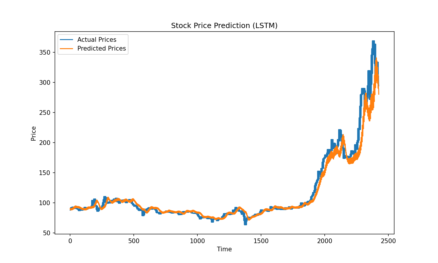
73: plt.savefig('images/stock-lstm-predict.png', dpi=150)
74: plt.show()
4.2. 能怎麼胡搞
- 多讀些原始資料
- 用更多特徵值來預測
- 用更多/更少天數來預測
- 變更模型架構
- 變更訓練集:測試集比例
- 增加epoch